Note: This report is presented as an interactive IPython notebook. Code and text are presented concurrently, to provide examples and code blocks alongside explanations.
# import statements
import osmnx as ox
import networkx as nx
import time
from IPython.display import IFrame
import folium

%matplotlib inline
ox.config(log_file=True, log_console=True, use_cache=True)
Introduction
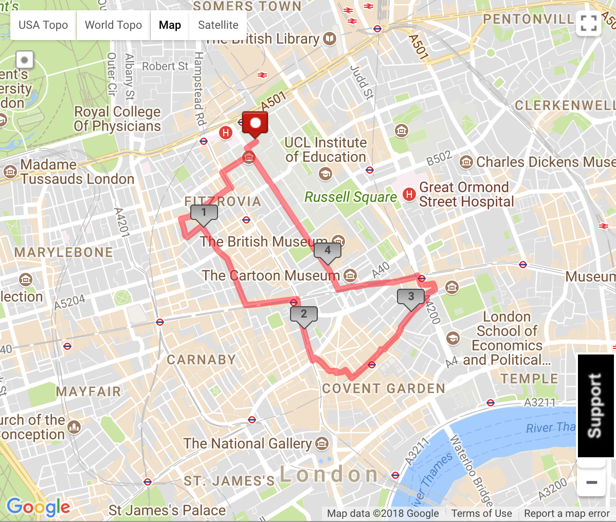
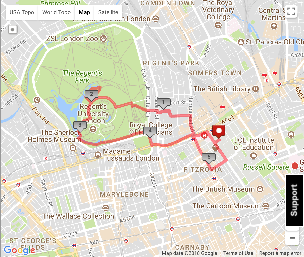
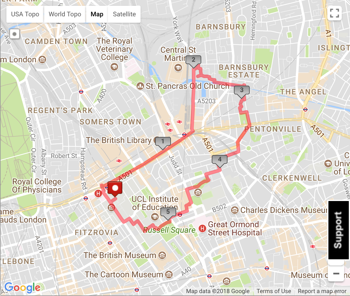
Today’s runner is more tech savvy than ever. Armed with GPS-enabled Garmin and Apple watches and shoe-embedded sensors, runners can track in real time everything from pace to heart rate to foot strike angle. A myriad of apps and websites exist to help them analyze this data: MapMyRun, Strava, MyFitnessPal, etc. Many of these tools help runners discover routes through crowd-sourced databases or randomly generating routes of a given length from a user-specified start point. Given the proliferation of GPS-enabled fitness services, it is no wonder that a number of patents have been filed for route suggestion engines [1; 2; 3].
 |
 |
 |
|---|---|---|
| Route 1 | Route 2 | Route 3 |
Visit MapMyRun to make your own.
Despite the data available to these tools - in some cases, a person’s complete running history - route suggestion engines do not take advantage of prior run data to suggest novel routes. This coursework aims to rectify that deficiency by creating a route engine that uses past GPX tracks to prioritize never before traveled segments of road, encouraging a runner to explore new areas.
This paper details the design and implementation process of a novel route generation algorithm. It addresses the assuptions made and the software packages used for development. It describes the core route generation and walks through a full example. An evaluation of algorithm performance is provided. Finally, following a brief discussion, suggestions are made for further research and development.
Note: In this paper, “road segment” will refer to a single stretch of road, trail, path, way, etc between two intersections. A road comprises one or more road segments.
Design
To prototype this novel route generator, I modified the sourcode of the OSMnx package, including the addition of two new modules and over 900 lines of code. This open-source code adds additional functionality to OSMnx allowing programmers to read and parse GPX tracks and create looped routes.
This section describes the design of this project, including the assumptions made, packages used, function architecture, and roadblocks encountered. Where possible, links are provided to specific implementations in code.
Assumptions
In the course of building out this project, a number of design decisions have been made to simplify the problem or reduce ambiguity for the user:
- To preserve runner experience, some provisions have been made to reduce number of turns.
- To avoide routes that are both challenging to navigate and frustraing to run, edges that minimize turns are prioritized.
- See:
osmnx/gpx.py:237
- All traveled roads are weighted the same.
- A road segment does not receive an additional penalty for being frequently run and is as likely to be run again as a road segment that has only been traveled once before.
- See:
osmnx/gpx.py:251
- Dead ends are avoided where possible.
- Cul-de-sacs and other dead ends are avoided, no matter how long they are. While this does exclude viable routes where the dead end path could provide a long out-and-back, it avoids short (and annoying) additions. Unfortunately this dataset contains some erroneous nodes that make avoiding all dead ends difficult.
- See:
osmnx/gpx.py:157
- Distance tolerance is a user-defined variable.
- As it is nearly impossible to create a route of exactly the desired distance, users may specify the tolerance for the desired distance. The greater the tolerance, the more routes can be generated. Too small of a tolerance may result in no routes at all.
- See:
osmnx/gpx.py:393
Software Packages
This project is built in Python 3.5 using the packages NetworkX and OSMnx.
NetworkX is an open source package designed to help researchers load, render, manipulate, and query large networks [4].
Open Street Map NetworkX (OSMnx) is built on top of NetworkX and provides explicit handling of spatial networks. It includes functionality to download portions of road network via the Open Street Map API and display maps as static images or Folium web maps in addition to spatial query functionality [5].
Most functions created as part of this coursework were built in package extensions to OSMnx through the osmnx/route.py and osmnx/gpx.py modules. The full amended code, including inline documentation, is availabile via this GitHub Fork.
See Appendix: Installation for information on how to install and use this package.
Functional Architecture
Designing this system required addressing three primary tasks map matching, route generation, and rendering results.
Map Matching
Map matching is the process of snapping location points obtained through GPS to a road segments. For our application, this is crucial: it allows traversed OSM road segments to be identified from GPX files. However, this is a challenging task. A single GPS point may be located on a road segment, equidistant from two or more segments, or not sufficiently close to any existing segment.
To address the challenge of matching GPX points to road networks, engineers at Microsoft developed the ST Matching algorithm [6]. This has been incorporated into the Open Source Routing Machine API, an open source project dedicated to making routing and location information available [7].
For this project, map matching is implemented in osmnx/gpx.py, which parses GPX tracks using Python package gpx-py [8]. These parsed tracks may be passed through Open Source Routing Machine API to get OSM Node IDs. Once GPX tracks have been matched to OSM road segments, each segment is assigned a frequency attribute based on how often it has been traversed (see osmnx/gpx.py:267). This attribute is used in the route generation algorithm.
The cells below read in a folder of GPX tracks, convert them to a dictionary of traversed paths, and return that dictionary. The parameter npoints refers to the number of points per track that are fed into the API. If npoints exceeds the number of points in the track, the points are uniformly sampled. Values between 100-400 seem to return reasonable results.
# read in folder of gpx track and return dictionary of points
folder = "london/"
sample_freq = ox.freq_from_folder(folder,npoints=199)
# show example of first 5 entries
print(dict(list(sample_freq.items())[0:6]))
Unfortunately this matching has proved difficult as the Open Source Routing Machine API cannot handle requests at the density provided by gpx tracks, and occasionally gets overloaded if it recieves requests too quickly. In addition, the OSM IDs used as keys in the above dictionary (sample_freq) do not always match up with the OSMIDs retained by the simplified graph. However, these frequency counts provide a starting point for the development of the route generation algorithm.
Route Generation Algorithm
The route generation algorithm is the brain of this project, primarily executed by the function generate_route (see osmnx/route.py:375). Following the approach taken by Leigh M. Chinitz [1], route generation is broken into two phases: outbound routing and inbound routing.
Both phases use a greedy heuristic to determine which edge to take next from a given node. From the current node (or starting node), the algorithm evaluates the 'suitability' of each adjacent edge based on their properties, such as length, bearing/orientation, and frequency of traversal. These suitability scores are stored in a vector of length equal to the number of evaluated nodes. They are then normalized such that all scores add to one and an edge is chosen at random with probability corresponding to the normalized suitability score.
| Candidate 1 | Candidate 2 | Candidate 3 | Candidate 4 | |
|---|---|---|---|---|
| Suitability Score | 4 | 5 | 10 | 1 |
| Normalized Suitability Score | 0.2 | 0.25 | 0.5 | 0.05 |
| Selected Edge | x |
The edge is selected randomly, with probability equal to the normalized suitability score.
Once the next edge has been selected, the end node of that edge becomes the current node.
Importantly, this process is not determininistic, allowing the user to obtain a different result every time the algorithm is run (see osmnx/route.py:201).
Outbound Phase
In the outbound phase, edges are prioritized based on similarity to previous orientation (preventing frequent turns), difference from bearing to home (preventing the runner from passing the start point mid-route), if been traversed before ever, if it has been traversed on this run, and on length (see osmnx/route.py:211).
Each of these values is scaled between 1-10 and given an importance weighting. These are then multiplied and summed, providing a ranking between 1 and 10 per edge considered. Variables that correspond to route quality, such as previous bearing, have high weightings to increase the "runnability" of the route.
| Variable | Explanation | Value Range | Weight | Example Value |
|---|---|---|---|---|
previous_bearing |
Prevent frequent turns | 0-180 | 0.3 | 5 |
home_bearing |
Prevent heading towards home too soon | 0-180 | 0.3 | 4 |
traveled |
Is this edge already in this route? | Boolean | 0.25 | 10 |
freq |
Has this edge been run before? | Boolean | 0.1 | 10 |
length |
How long is the road segment? | > 0 | 0.05 | 10 |
| Example Edge | Score | 6.7 |
These variables and weights were chosen for convenience. Further work should evalute more rigorous choices for the weights, variables chosen, and the suitability function itself (here, a simple weighted average).
The outbound phase is run until the total route length has reached half of the goal length.
Inbound Phase
Much like the outbound phase, the inbound phase uses a weighted average to calculate edge suitability. However, this weighted average is adaptive and gives greater priority to homeward bound edges as the route length becomes closer to the goal length (see osmnx/route.py:292).
The table below shows an evaluation for a homebound node where pct_remaining (% of the goal length remaining) is 10%.
| Variable | Explanation | Value Range | Weight | Example Value |
|---|---|---|---|---|
previous_bearing |
Prevent frequent turns | 0-180 | 0.3 * pct_remaining |
5 |
home_bearing |
Encourage heading towards | 0-180 | (1 - pct_remaining) |
4 |
traveled |
Is this edge already in this route? | Boolean | 0.25 * pct_remaining |
10 |
freq |
Has this edge been run before? | Boolean | 0.1 * pct_remaining |
10 |
length |
How long is the road segment? | > 0 | 0.05 * pct_remaining |
10 |
| _Example Edge_ | Score | 4.15 |
To ensure that all routes are able to reach home, at each step the shortest distance home is calculated using a function from the NetworkX package.
If the route length plus the shortest distance home is less than goal_length - 0.5*tolerance, additional edges are added to the route using the weighted average described above (see osmnx/route.py:472). Tolerance can be specified by the user; in these examples, tolerance was set at 0.5km.
However, if route length plus the shortest distance home is greater than goal_length - 0.5*tolerance but less than goal_length + tolerance, the algorithm is forced to return to the start point immediately via the shortest path (see osmnx/route.py:486).
If no route can be found to accomplish this return home, the function returns a warning and a list containing only the start node (that is, it fails to find or return a route; see osmnx/route.py:492).
Finally, route is returned as a list of nodes traversed in order.
Rendering Results
Rendering results is vital to communicate the chosen route to the user. Using built in OSMnx functionality, the suggested route is plotted on top of the local street network in a Folium webmap. The start/end node is marked by a popup containing metadata about route novelty and distance.
Route opacity is used to emphasize route nodes as well as segments that are traversed more than once in the same route.
example_route = 'data/example_route_1524767198.html'
IFrame(example_route, width=900, height=500)
Click on the white marker in the map above to see information about the route!
Example
This section shows a full example, from generation of the frequency dictionary to plotting the route in an interactive webmap. Running this section again should result in a different route every time!
Note: this code is very much still in development, and as such contains an number of bugs! If you receive an error trying to run this process, especially in the function ox.generate_route, simply re-run a few times - the algorithm is not likely to pick two or three bad routes in a row.
# parameters for our route
start_lat = 51.522462 # start point near UCL campus
start_lon = -0.132630
goal_length = 5 # in km
freq_folder = 'london/' # relative path of folder of gpx tracks, or leave as empty string

# parameters for our visualization
route_color = '#7be1ed'
icon_color = '#00d1ea'
map_tiles = 'CartoDB dark_matter'
# get frequency dictionary
freq = ox.freq_from_folder(freq_folder,npoints=250)
# create street map around our start point
streets = ox.graph_from_point((start_lat, start_lon),
                              distance=goal_length*1000/1.75, network_type='walk')
# create a route!
newroute = ox.generate_route(start_lat, start_lon, goal_length, graph=streets)
# get metrics about route novelty to add to map
novel_segments, novel_length = ox.novelty_score(streets, newroute)
route_length = ox.total_route_length(streets, newroute)
message = '{:0.1f}km route containining {}/{} novel segments \
           (novelty: {:0.1f}km, {:0.1f}% of total length)'.format(route_length/1000,
                                     novel_segments,len(newroute)-1,
                                     novel_length/1000,100*novel_length/route_length)
# plot the route with folium on top of the previously created graph_map
route_graph_map = ox.plot_route_folium(streets, newroute,
                                       route_opacity=0.5,
                                       tiles = map_tiles,
                                       route_color = route_color)
# add start/endpoint marker
folium.Marker([start_lat, start_lon], popup=message,
              icon=folium.Icon(color='white',icon_color=icon_color,icon='child',
                             prefix='fa')).add_to(route_graph_map)
# save as html file then display map in IPython as an iframe
filepath = 'data/example_route_{:0.0f}.html'.format(time.time())
route_graph_map.save(filepath)
IFrame(filepath, width=800, height=500)
Performance
Ideally, this type of algorithm would be optimized to be used in real time: a user could open their Strava or MapMyRun homepage and simplly click a point on the map to generate a brand new route. Consequently, minimizing runtime is crucial.
| Step | Source | Runtime(s) | Notes |
|---|---|---|---|
| Frequency Generator (1 file) | OSMNx gpx (custom) | 0.11728 | This depends in part on the file size, number of points sent to the server, whether the request has been cached or not, etc. |
| Frequency Generator (13 files) | OSMNx gpx (custom) | 3.46759 | |
| Create Base Graph (2.86km radius) | OSMnx Core | 26.90495 | Simplifying OSM data to a "clean" graph containing nodes only at intersections or dead ends is time intensive. |
| Create Base Graph (5.72km radius) | OSMnx Core | 76.08142 | Speed also depends on whether the request has been cached, how complicated the graph is, and how busy the OSM server is. |
| Create Route (5km goal length) | OSMnx Routing (custom) | 4.04785 | |
| Create Route (10km goal length) | OSMnx Routing (custom) | 9.26532 | This indicates that routefinding time may scale linearly. |
| Create + Display Webmap (10km) | OSMnx Core + OSMnx Routing (custom) | 9.99639 | In a web application, the route would be rendered atop an existing map, saving time. |
Future work should provide more rigorous benchmarking and time profiling of these functions.
As the table above shows, the core algorithm takes around ~4 seconds for a 5km route and ~9 seconds for a 10km route. The largest time requirements are for creating the base graph, which may take over a minute to retrieve from the server and simplify depending on street density and radius. This could be pre-loaded in a browser or cached, dramatically reducing the time required to generate a route.
No explicit steps were taken in the course of this project to optimize algorithm performance. Future work on this project would necessarily take a much more rigorous approach to benchmarking the runtime of these different steps.
Discussion
As demonstrated above, the algorithm created in this coursework is capable of creating random running routes given particular priorities. Implemented as modules within the OSMnx library, this algorithm takes advantage of open source software to model, compute, and render routes of arbitrary length. We discuss bugs, runner experience fixes, and potential improvements to the work herein presented.
A number of bugs remain within the code:
- Map matching of GPX tracks occasionally fails due to miscommunication with the server.
- Map matched edges may or may not be present in the simplified graph used for routing, leading to incorrect estimates of which road segments have been traversed.
- One common error is
, indicating that no edges exist from which to choose. This typically occurs when a route accidently heads down an improperly simplified dead end.
A number of improvements can be made to improve runner experience, or how high of quality runners percieve these routes to be:
- Eliminate complicated intersection crossings, perhaps using the the OSMnx
clean_intersectionsfunctionality. - Eliminate self-crossing of routes, which can be disorienting for some runners.
In addition to these improvements, the core of the route creation algorithm would benefit from increased mathematical rigor. While a simple greedy heuristic using a weighted average is a sufficient starting point for this prototype, a more sophisticated mathematical model taking into account multiple areas of the graph as well as past behavior would lend rigor to this interesting problem. Future improvements should also focus on runtime reduction, with the objective of achieving near real-time in-brower speeds.
Finally, I believe developers who benefit from open source software have an obligation to give back to the community. Many of the functions developed as part of this project could, with additional bug-fixes, be incorporated back into the core OSMnx package.
Conclusion
As runners and other exercise enthusiasts continue to collect data, companies such as Strava and MapMyRun will race to extract insight and provide value back to users from this data. In this field, novel exercise route generation is an exciting and potentially lucrative computational networks problem.
This project has demonstrated a basic prototype for creating such routes based on the open source Python package OSMnx, including map matching of GPX tracks to derive frequency information. Future implementations of this project could aim to reduce bug fixes, improve performance, increase route quality, and contribute back to the open source community.
References
[1] Chinitz, L. M. 2004. Travel route mapping, US7162363B2.
[2] Brooks, A. 2005. Route based on distance, US20060206258A1.
[3] Van Hende, I. 2010. Method of creating customized exercise routes for a user, US20120143497A1.
[4] Hagberg, A., Schult, D., and Swart, P. 2008. “Exploring network structure, dynamics, and function using NetworkX” Proceedings of the 7th Python in Science Conference (SciPy2008), Gäel Varoquaux, Travis Vaught, and Jarrod Millman (Eds), (Pasadena, CA USA), pp. 11–15.
[5] Boeing, G. 2017. "OSMnx: New Methods for Acquiring, Constructing, Analyzing, and Visualizing Complex Street Networks." Computers, Environment and Urban Systems 65, 126-139. doi:10.1016/j.compenvurbsys.2017.05.004
[6] Lou, Y., Zhang, C., Zheng, Y., Xie, X., Wang, W. and Huang, Y., 2009, November. Map-matching for low-sampling-rate GPS trajectories. In Proceedings of the 17th ACM SIGSPATIAL international conference on advances in geographic information systems (pp. 352-361). ACM.
[7] Open Source Routing Machine. Accessed at: http://project-osrm.org/.
[8] gpx-py. Accessed at: https://github.com/tkrajina/gpxpy.
Appendix
Installation
To run the code examples in this notebook from scratch, or to explore other functionality built out in the route and gpx modules of OSMnx, clone or download my fork of the OSMnx package locally.
git clone git@github.com:heidimhurst/osmnx.git
Install OSMnx from scratch in a brand new virtual environment using Conda. Installation using the Conda Forge package ensures that correct dependencies are all installed as well.
conda create --override-channels -c conda-forge -n OSMNX python=3 osmnx
Activate the virtual environment, and overwrite the original OSMnx package with the downloaded version of my code.
source activate OSMNX
pip install -e ~/{path_to_downloaded_fork}/osmnx
You can then use OSMnx, including my modifications, from a Python script or IPython notebook while in this virtual environment.